3. Performance Benchmark with other packages
Source:vignettes/fundiversity_2-performance.Rmd
fundiversity_2-performance.RmdThis vignette presents some performance tests ran between
fundiversity and other functional diversity packages. Note
that to avoid the dependency on other packages, this vignette is pre-computed.
Other packages to compute FD indices
Main functions
Here is a table that summarizes the comparable functions (and their
arguments) for functions included in fundiversity. Note
that the package name is indicated before :: followed by
the function name.
| Index Type | Index Name | Source |
fundiversity function |
Equivalent Functions |
|---|---|---|---|---|
| α-diversity | Functional Dispersion (FDis) | Laliberté and Legendre (2010) | fd_fdis() |
BAT::dispersion()FD::fdisp()hillR::hill_func()FD for FDis computations and standardize
the traits without telling the
user)mFD::alpha.fd.multidim(..., ind_vect = "fdis")
|
| α-diversity | Functional Divergence (FDiv) | Villéger, Mason, and Mouillot (2008) | fd_fdiv() |
mFD::alpha.fd.multidim(..., ind_vect = "fdiv") |
| α-diversity | Functional Evenness (FEve) | Villéger, Mason, and Mouillot (2008) | fd_feve() |
mFD::alpha.fd.multidim(..., ind_vect = "feve") |
| α-diversity | Functional Richness (FRic) | Villéger, Mason, and Mouillot (2008) | fd_fric() |
BAT::alpha() (tree, not strictly
equal)BAT::hull.alpha()
(hull)mFD::alpha.fd.multidim(..., ind_vect = "fric")
|
| α-diversity | Rao’s Quadratic Entropy (Q) | Villéger, Grenouillet, and Brosse (2013) | fd_raoq() |
adiv::QE()BAT::rao()hillR::hill_func()
(standardize traits without
warning)mFD::alpha.fd.hill(..., q = 2, tau = "max")
(returns a slightly modified version of Q according to Ricotta and Szeidl (2009)) |
| β-diversity | Functional Richness Intersection (FRic_intersect) | Rao (1982) | fd_fric_intersect() |
betapart::functional.beta.pair()hillR::hill_func_parti_pairwise()
|
The other packages are thus: adiv (Pavoine 2020), BAT (Cardoso, Rigal, and Carvalho 2015),
betapart (Baselga and Orme
2012), FD (Laliberté,
Legendre, and Shipley 2014), hillR (Li 2018), and mFD (Magneville et al. 2022). For fairness of
comparison, even if FD::dbFD() contains most indices we’re
not considering it as it computes all indices together for each call,
and would necessarily be slower.
Benchmark between packages
We will now benchmark the functions included in
fundiversity with the corresponding function in other
packages using the microbenchmark::microbenchmark()
function. We will use the fairly small (~220 species, 8 sites, 4 traits)
provided dataset in fundiversity.
tictoc::tic()  # Time execution of vignette
library(fundiversity)
data("traits_birds", package = "fundiversity")
data("site_sp_birds", package = "fundiversity")

dist_traits_birds <- dist(traits_birds)
Functional Dispersion (FDis)
fdis_bench <- microbenchmark::microbenchmark(
  fundiversity = {
    fundiversity::fd_fdis(traits_birds, site_sp_birds)
  },
  FD = {
    FD::fdisp(dist_traits_birds, site_sp_birds)
  },
  mFD = {
    mFD::alpha.fd.multidim(
    traits_birds, site_sp_birds, ind_vect = "fdis",
    scaling = FALSE, verbose = FALSE, details_returned = FALSE
  )
  },
  times = 30
)

ggplot2::autoplot(fdis_bench) +
  labs(title = "Functional Dispersion (FDis)")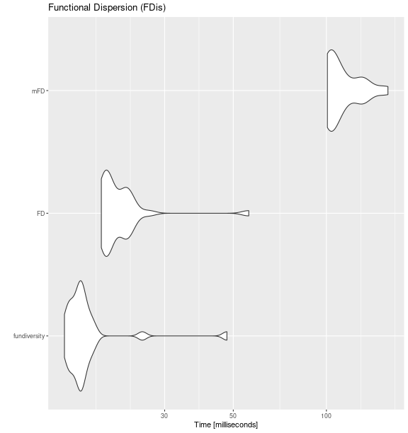
Functional Divergence (FDiv)
fdiv_bench <- microbenchmark::microbenchmark(
  fundiversity = fd_fdiv(traits_birds, site_sp_birds),
  mFD = mFD::alpha.fd.multidim(
    traits_birds, site_sp_birds, ind_vect = "fdiv",
    scaling = FALSE, verbose = FALSE
  ),
  times = 30
)

ggplot2::autoplot(fdiv_bench) +
  labs(title = "Functional Divergence (FDiv)")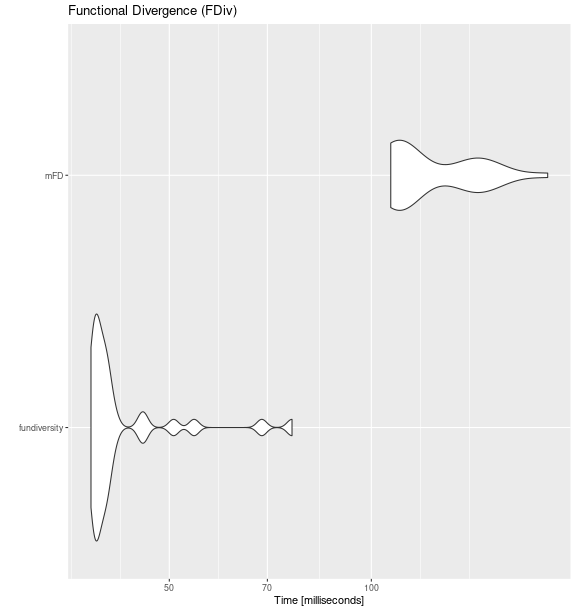
Functional Evenness (FEve)
feve_bench <- microbenchmark::microbenchmark(
  fundiversity = fd_feve(traits_birds, site_sp_birds),
  mFD = mFD::alpha.fd.multidim(
    traits_birds, site_sp_birds, ind_vect = "feve",
    scaling = FALSE, verbose = FALSE
  ),
  times = 30
)

ggplot2::autoplot(feve_bench) +
  labs(title = "Functional Evenness (FEve)")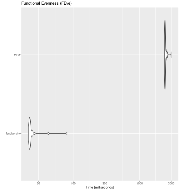
Functional Richness (FRic)
fric_bench <- microbenchmark::microbenchmark(
  fundiversity = fd_fric(traits_birds, site_sp_birds),
  BAT_tree = BAT::alpha(
    site_sp_birds, traits_birds
  ),
  BAT_alpha_hull = BAT::hull.alpha(
    BAT::hull.build(site_sp_birds, traits_birds)
  ),
  mFD = mFD::alpha.fd.multidim(
    traits_birds, site_sp_birds, ind_vect = "fric",
    scaling = FALSE, verbose = FALSE
  ),
  times = 30
)

ggplot2::autoplot(fric_bench) +
  labs(title = "Functional Richness (FRic)")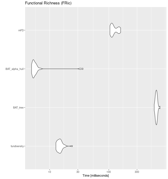
Functional Richness Intersection (FRic_intersect)
fric_bench <- microbenchmark::microbenchmark(
  fundiversity  = fd_fric_intersect(traits_birds, site_sp_birds) ,
  betapart = betapart::functional.beta.pair(
    site_sp_birds, traits_birds
  ),
  hillR = hillR::hill_func_parti_pairwise(
    site_sp_birds, traits_birds, .progress = FALSE
  ),
  times = 30
)

ggplot2::autoplot(fric_bench) +
  labs(title = "Functional Richness Intersection (FRic)")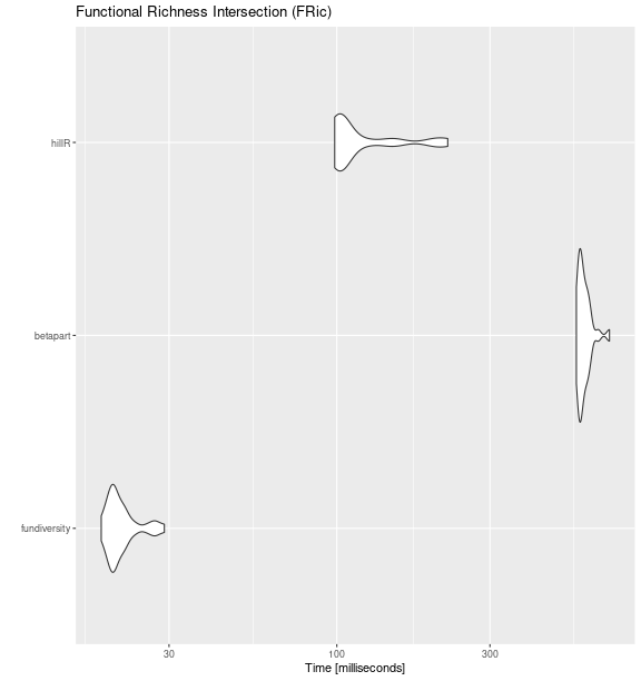
Rao’s Quadratic Entropy (Q)
raoq_bench <- fric_bench <- microbenchmark::microbenchmark(
  fundiversity = fd_raoq(traits_birds, site_sp_birds),
  adiv= adiv::QE(
    site_sp_birds, dist_traits_birds
  ),
  BAT_rao           = BAT::rao(
    site_sp_birds, distance = traits_birds
  ),
  hillR_hill_func   = hillR::hill_func(
    site_sp_birds, traits_birds, fdis = FALSE
  ),
  mFD_alpha_fd_hill = mFD::alpha.fd.hill(
    site_sp_birds, dist_traits_birds, q = 2,
    tau = "max"
  ),
  times = 30
)

ggplot2::autoplot(raoq_bench) +
  labs(title = "Rao's Quadatric Entropy (Q)")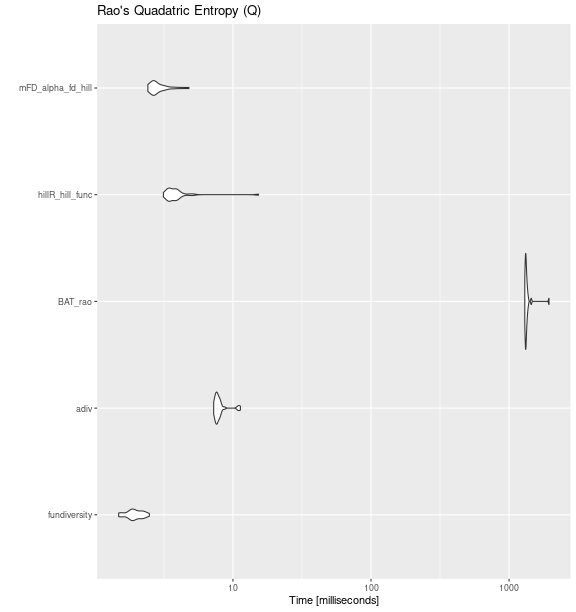
Benchmark within fundiversity
We now proceed to the performance evaluation of functions within
fundiversity with datasets of increasing sizes.
Increasing the number of species
make_more_sp <- function(n) {
  traits <- do.call(rbind, replicate(n, traits_birds, simplify = FALSE))
  row.names(traits) <- paste0("sp", seq_len(nrow(traits)))

  site_sp <- do.call(cbind, replicate(n, site_sp_birds, simplify = FALSE))
  colnames(site_sp) <- paste0("sp", seq_len(ncol(site_sp)))

  list(tr = traits, si = site_sp)
}

null_sp_1000   <- make_more_sp(5)
null_sp_10000  <- make_more_sp(50)
null_sp_100000 <- make_more_sp(500)
Functional Richness
bench_sp_fric <- microbenchmark::microbenchmark(
  species_200    = fd_fric(     traits_birds, site_sp_birds),
  species_1000   = fd_fric(  null_sp_1000$tr, null_sp_1000$si),
  species_10000  = fd_fric( null_sp_10000$tr, null_sp_10000$si),
  species_100000 = fd_fric(null_sp_100000$tr, null_sp_100000$si),
  times = 30
)

ggplot2::autoplot(bench_sp_fric)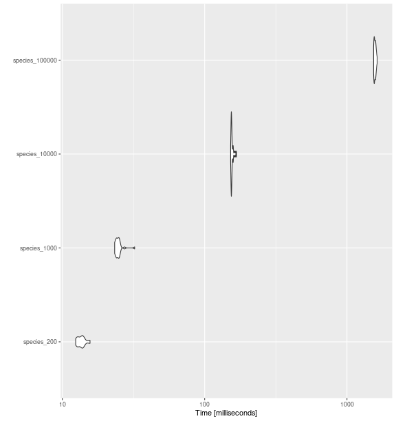
fd_fric()
with increasing number of species.
bench_sp_fric
#> Unit: milliseconds
#>            expr        min         lq       mean     median         uq        max neval  cld
#>     species_200   12.40461   12.86473   13.63794   13.65822   13.96949   15.64313    30 a
#>    species_1000   23.31024   23.98235   24.77462   24.52898   24.99526   32.20389    30  b
#>   species_10000  152.16972  153.69475  155.65197  154.41463  155.87235  167.39586    30   c
#>  species_100000 1538.24210 1552.02784 1573.05390 1571.92017 1587.70159 1629.76043    30    d
Functional Divergence
bench_sp_fdiv <- microbenchmark::microbenchmark(
  species_200    = fd_fdiv(     traits_birds, site_sp_birds),
  species_1000   = fd_fdiv(  null_sp_1000$tr, null_sp_1000$si),
  species_10000  = fd_fdiv( null_sp_10000$tr, null_sp_10000$si),
  species_100000 = fd_fdiv(null_sp_100000$tr, null_sp_100000$si),
  times = 30
)

ggplot2::autoplot(bench_sp_fdiv)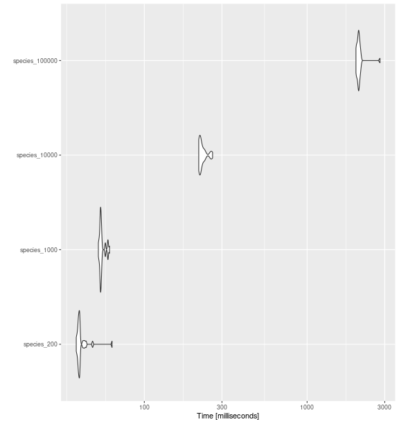
fd_fdiv()
with increasing number of species.
bench_sp_fdiv
#> Unit: milliseconds
#>            expr        min         lq       mean     median         uq        max neval cld
#>     species_200   38.18281   39.33241   41.03782   39.80735   40.19474   63.38092    30 a
#>    species_1000   52.21140   53.58856   54.88775   54.00482   54.58979   61.12244    30 a
#>   species_10000  215.96505  218.21261  227.32449  221.46767  231.33971  262.64920    30  b
#>  species_100000 1996.22764 2035.16809 2090.07993 2068.75306 2097.02749 2805.37816    30   c
Rao’s Quadratic Entropy
bench_sp_raoq <- microbenchmark::microbenchmark(
  species_200    = fd_raoq(     traits_birds, site_sp_birds),
  species_1000   = fd_raoq(  null_sp_1000$tr, null_sp_1000$si),
  species_10000  = fd_raoq( null_sp_10000$tr, null_sp_10000$si),
  times = 30
)

ggplot2::autoplot(bench_sp_raoq)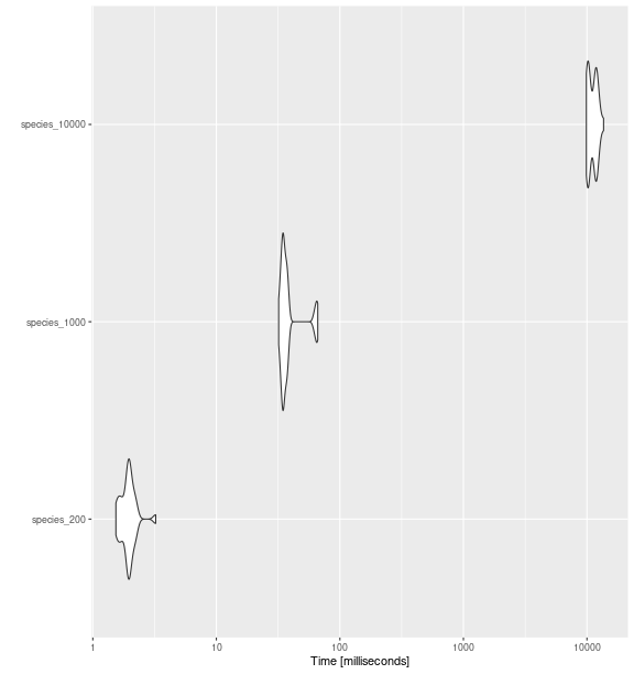
fd_raoq()
with increasing number of species.
bench_sp_raoq
#> Unit: milliseconds
#>           expr         min           lq         mean       median           uq          max neval cld
#>    species_200    1.537703     1.751935     1.954434     1.950017     2.041037     3.230497    30  a
#>   species_1000   31.957110    34.274255    39.128452    35.156704    37.556228    66.194976    30  a
#>  species_10000 9890.756358 10163.144236 11121.366410 11055.979331 11964.694993 13632.668874    30   b
Functional Evenness
bench_sp_feve <- microbenchmark::microbenchmark(
  species_200    = fd_feve(     traits_birds, site_sp_birds),
  species_1000   = fd_feve(  null_sp_1000$tr, null_sp_1000$si),
  species_10000  = fd_feve( null_sp_10000$tr, null_sp_10000$si),
  times = 15
)

ggplot2::autoplot(bench_sp_feve)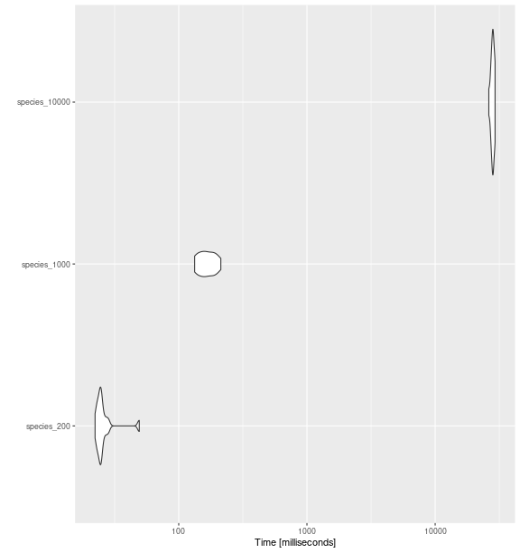
fd_feve()
with increasing number of species.
bench_sp_feve
#> Unit: milliseconds
#>           expr         min          lq        mean      median          uq         max neval cld
#>    species_200    22.25434    23.58857    26.28398    24.66652    25.41282    49.21613    15  a
#>   species_1000   133.12192   148.39296   167.29508   163.98844   186.30949   212.94652    15  a
#>  species_10000 26209.90991 27553.75296 28085.39492 28186.57578 28599.03918 29311.05335    15   b
Comparing between indices
all_bench_sp <- list(fric = bench_sp_fric,
                     fdiv = bench_sp_fdiv,
                     raoq = bench_sp_raoq,
                     feve = bench_sp_feve) %>%
  bind_rows(.id = "fd_index") %>%
  mutate(n_sp = gsub("species_", "", expr) %>%
           as.numeric())

all_bench_sp %>%
  ggplot(aes(n_sp, time * 1e-9, color = fd_index)) +
  geom_point(alpha = 1/3) +
  geom_smooth() +
  scale_x_log10() +
  scale_y_log10() +
  scale_color_brewer(type = "qual",
                     labels = c(fric = "FRic", fdiv = "FDiv", raoq = "Rao's Q",
                                feve = "FEve")) +
  labs(title = "Performance comparison between indices",
       x = "# of species", y = "Time (in seconds)",
       color = "FD index") +
  theme_bw() +
  theme(aspect.ratio = 1)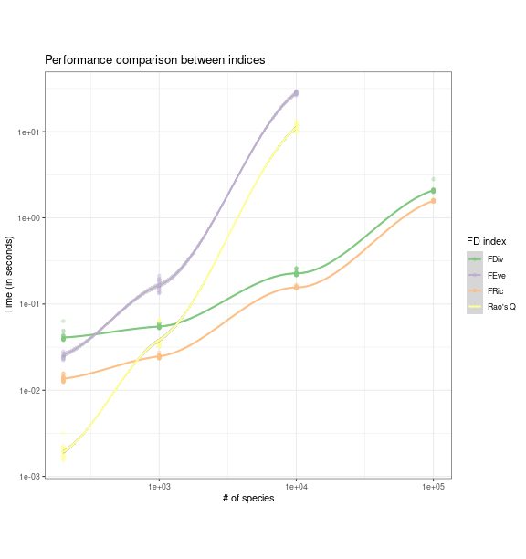
fundiversity with increasing number of
species. Smoothed trend lines and standard error envelopes ares
shown.Increasing the number of sites
make_more_sites <- function(n) {
  site_sp <- do.call(rbind, replicate(n, site_sp_birds, simplify = FALSE))
  rownames(site_sp) <- paste0("s", seq_len(nrow(site_sp)))

  site_sp
}

site_sp_100   <- make_more_sites(12)
site_sp_1000  <- make_more_sites(120)
site_sp_10000 <- make_more_sites(1200)
Functional Richness
bench_sites_fric <- microbenchmark::microbenchmark(
  sites_10    = fd_fric(traits_birds, site_sp_birds),
  sites_100   = fd_fric(traits_birds, site_sp_100),
  sites_1000  = fd_fric(traits_birds, site_sp_1000),
  sites_10000 = fd_fric(traits_birds, site_sp_10000),
  times = 15
)

ggplot2::autoplot(bench_sites_fric)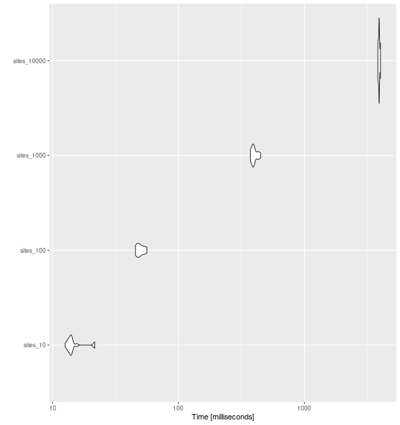
fd_fric()
with increasing number of sites.
bench_sites_fric
#> Unit: milliseconds
#>         expr        min         lq       mean     median         uq        max neval  cld
#>     sites_10   12.60195   13.45944   14.88054   13.96007   14.29602   21.66510    15 a
#>    sites_100   45.57530   47.25923   49.87524   48.75620   52.29567   56.19952    15  b
#>   sites_1000  372.72833  386.35628  400.43169  395.60903  408.99573  449.87164    15   c
#>  sites_10000 3833.05136 3885.11306 3921.60544 3919.29055 3942.32492 4016.96576    15    d
Functional Divergence
bench_sites_fdiv <- microbenchmark::microbenchmark(
  sites_10    = fd_fdiv(traits_birds, site_sp_birds),
  sites_100   = fd_fdiv(traits_birds, site_sp_100),
  sites_1000  = fd_fdiv(traits_birds, site_sp_1000),
  sites_10000 = fd_fdiv(traits_birds, site_sp_10000),
  times = 15
)

ggplot2::autoplot(bench_sites_fdiv)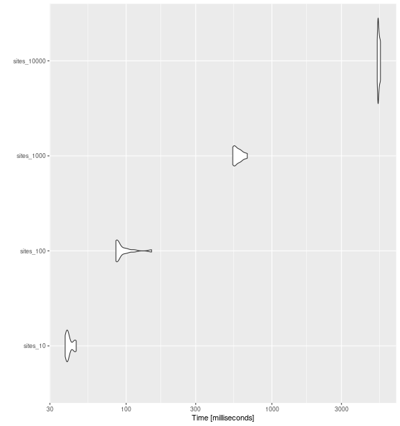
fd_fdiv()
with increasing number of sites.
bench_sites_fdiv
#> Unit: milliseconds
#>         expr        min         lq       mean     median         uq        max neval  cld
#>     sites_10   38.17040   39.17880   40.79484   39.59029   42.08936   45.43952    15 a
#>    sites_100   85.09805   85.99399   94.77048   86.88365   96.33675  149.45931    15  b
#>   sites_1000  538.76135  545.03628  582.84610  564.85683  605.87486  677.86382    15   c
#>  sites_10000 5278.55172 5336.69296 5405.90861 5378.53730 5458.24597 5552.26594    15    d
Rao’s Quadratic Entropy
bench_sites_raoq = microbenchmark::microbenchmark(
  sites_10    = fd_raoq(traits = NULL, site_sp_birds, dist_traits_birds),
  sites_100   = fd_raoq(traits = NULL, site_sp_100,   dist_traits_birds),
  sites_1000  = fd_raoq(traits = NULL, site_sp_1000,  dist_traits_birds),
  sites_10000 = fd_raoq(traits = NULL, site_sp_10000, dist_traits_birds),
  times = 15
)

ggplot2::autoplot(bench_sites_raoq)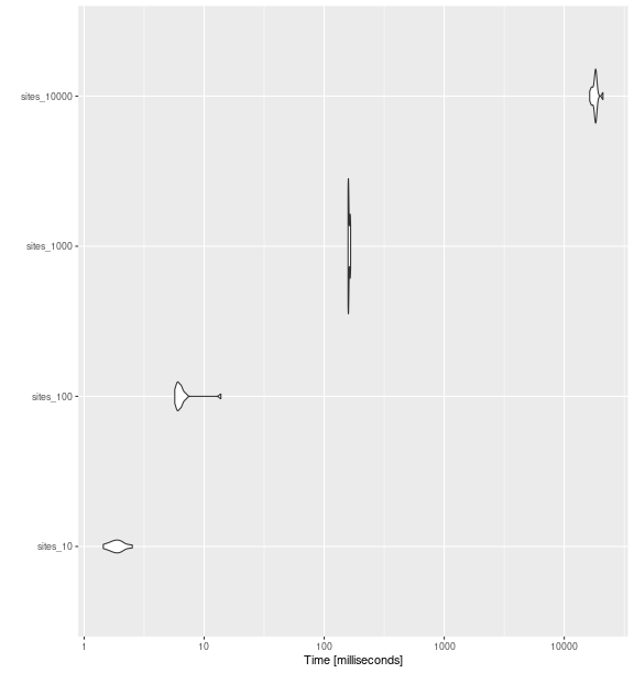
fd_raoq()
with increasing number of sites.
bench_sites_raoq
#> Unit: milliseconds
#>         expr          min           lq         mean       median           uq          max neval cld
#>     sites_10     1.443757     1.717630     1.887153     1.861230     2.037991     2.518933    15  a
#>    sites_100     5.689849     6.004428     6.718675     6.178415     6.460348    13.786219    15  a
#>   sites_1000   158.130064   158.814848   160.907719   159.296631   163.977418   166.066294    15  a
#>  sites_10000 16296.391504 17530.369693 18080.130808 18193.538354 18411.571843 21033.249202    15   b
Functional Evenness
bench_sites_feve <- microbenchmark::microbenchmark(
  sites_10    = fd_feve(traits = NULL, site_sp_birds, dist_traits_birds),
  sites_100   = fd_feve(traits = NULL, site_sp_100,   dist_traits_birds),
  sites_1000  = fd_feve(traits = NULL, site_sp_1000,  dist_traits_birds),
  sites_10000 = fd_feve(traits = NULL, site_sp_10000, dist_traits_birds),
  times = 15
)

ggplot2::autoplot(bench_sites_feve)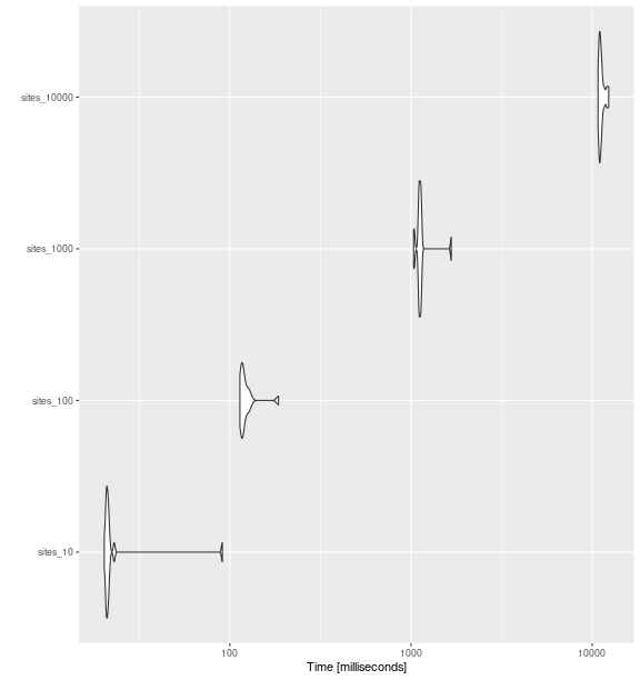
fd_feve()
with increasing number of sites
bench_sites_feve
#> Unit: milliseconds
#>         expr         min          lq        mean      median          uq         max neval cld
#>     sites_10    20.26885    20.79379    25.80265    21.06491    21.39182    90.92815    15 a
#>    sites_100   113.64419   115.81009   123.60943   118.04145   123.54457   185.57582    15 a
#>   sites_1000  1034.37573  1107.36408  1146.78358  1119.68000  1134.07348  1668.68480    15  b
#>  sites_10000 10779.65515 10969.94333 11249.27062 11090.00824 11317.37080 12341.22800    15   c
Comparing between indices
all_bench_sites <- list(fric = bench_sites_fric,
                        fdiv = bench_sites_fdiv,
                        raoq = bench_sites_raoq,
                        feve = bench_sites_feve) %>%
  bind_rows(.id = "fd_index") %>%
  mutate(n_sites = gsub("sites", "", expr) %>%
           as.numeric())

all_bench_sites %>%
  ggplot(aes(n_sites, time * 1e-9, color = fd_index)) +
  geom_point(alpha = 1/3) +
  geom_smooth() +
  scale_x_log10() +
  scale_y_log10() +
  scale_color_brewer(type = "qual",
                     labels = c(fric = "FRic", fdiv = "FDiv", raoq = "Rao's Q",
                                feve = "FEve")) +
  labs(title = "Performance comparison between indices",
       x = "# of sites", y = "Time (in seconds)",
       color = "FD index") +
  theme_bw() +
  theme(aspect.ratio = 1)
fundiversity with increasing number of
sites. Smoothed trend lines and standard error envelopes ares
shown.Session info of the machine on which the benchmark was ran and time it took to run
#>  seconds needed to generate this document: 1691.449 sec elapsed
#> ─ Session info ─────────────────────────────────────────────────────────────────────────────────────────────────────────────────────────────────
#>  setting  value
#>  version  R version 4.2.1 (2022-06-23)
#>  os       Ubuntu 20.04.5 LTS
#>  system   x86_64, linux-gnu
#>  ui       RStudio
#>  language (EN)
#>  collate  en_US.UTF-8
#>  ctype    en_US.UTF-8
#>  tz       Etc/UTC
#>  date     2022-11-15
#>  rstudio  2022.02.0+443 Prairie Trillium (server)
#>  pandoc   2.17.1.1 @ /usr/lib/rstudio-server/bin/quarto/bin/ (via rmarkdown)
#>
#> ─ Packages ─────────────────────────────────────────────────────────────────────────────────────────────────────────────────────────────────────
#>  package           * version    date (UTC) lib source
#>  abind               1.4-5      2016-07-21 [1] CRAN (R 4.2.0)
#>  ade4                1.7-19     2022-04-19 [1] CRAN (R 4.2.0)
#>  adegraphics         1.0-16     2021-09-16 [1] CRAN (R 4.2.1)
#>  adiv                2.2        2022-10-06 [1] CRAN (R 4.2.1)
#>  ape                 5.6-2      2022-03-02 [1] CRAN (R 4.2.0)
#>  assertthat          0.2.1      2019-03-21 [3] CRAN (R 4.1.3)
#>  base64enc           0.1-3      2015-07-28 [1] CRAN (R 4.2.1)
#>  BAT                 2.9.2      2022-11-08 [1] CRAN (R 4.2.1)
#>  betapart            1.5.6      2022-04-06 [1] CRAN (R 4.2.1)
#>  cachem              1.0.6      2021-08-19 [3] CRAN (R 4.1.3)
#>  caret               6.0-93     2022-08-09 [1] CRAN (R 4.2.1)
#>  class               7.3-20     2022-01-13 [5] CRAN (R 4.1.2)
#>  cli                 3.4.1      2022-09-23 [1] CRAN (R 4.2.1)
#>  cluster             2.1.3      2022-03-28 [5] CRAN (R 4.1.3)
#>  clusterGeneration   1.3.7      2020-12-15 [1] CRAN (R 4.2.0)
#>  coda                0.19-4     2020-09-30 [1] CRAN (R 4.2.0)
#>  codetools           0.2-18     2020-11-04 [5] CRAN (R 4.0.3)
#>  colorspace          2.0-3      2022-02-21 [1] CRAN (R 4.2.0)
#>  combinat            0.0-8      2012-10-29 [1] CRAN (R 4.2.0)
#>  crayon              1.5.1      2022-03-26 [1] CRAN (R 4.2.0)
#>  data.table          1.14.2     2021-09-27 [1] CRAN (R 4.2.0)
#>  DBI                 1.1.2      2021-12-20 [3] CRAN (R 4.1.3)
#>  deldir              1.0-6      2021-10-23 [1] CRAN (R 4.2.1)
#>  dendextend          1.16.0     2022-07-04 [1] CRAN (R 4.2.1)
#>  digest              0.6.29     2021-12-01 [1] CRAN (R 4.2.0)
#>  doParallel          1.0.17     2022-02-07 [1] CRAN (R 4.2.1)
#>  doSNOW              1.0.20     2022-02-04 [1] CRAN (R 4.2.1)
#>  dplyr             * 1.0.10     2022-09-01 [1] CRAN (R 4.2.1)
#>  e1071               1.7-12     2022-10-24 [1] CRAN (R 4.2.1)
#>  ellipsis            0.3.2      2021-04-29 [1] CRAN (R 4.2.0)
#>  evaluate            0.18       2022-11-07 [1] CRAN (R 4.2.1)
#>  expm                0.999-6    2021-01-13 [1] CRAN (R 4.2.0)
#>  fansi               1.0.3      2022-03-24 [1] CRAN (R 4.2.0)
#>  farver              2.1.0      2021-02-28 [1] CRAN (R 4.2.0)
#>  fastcluster         1.2.3      2021-05-24 [1] CRAN (R 4.2.1)
#>  fastmap             1.1.0      2021-01-25 [1] CRAN (R 4.2.1)
#>  fastmatch           1.1-3      2021-07-23 [1] CRAN (R 4.2.0)
#>  FD                  1.0-12.1   2022-05-02 [1] CRAN (R 4.2.0)
#>  foreach             1.5.2      2022-02-02 [1] CRAN (R 4.2.1)
#>  fundiversity      * 0.2.1.9000 2022-04-12 [3] Github (bisaloo/fundiversity@87652ba)
#>  future              1.28.0     2022-09-02 [1] CRAN (R 4.2.1)
#>  future.apply        1.10.0     2022-11-05 [1] CRAN (R 4.2.1)
#>  generics            0.1.2      2022-01-31 [1] CRAN (R 4.2.0)
#>  geometry            0.4.6      2022-04-18 [1] CRAN (R 4.2.0)
#>  ggplot2           * 3.3.6      2022-05-03 [1] CRAN (R 4.2.0)
#>  globals             0.16.1     2022-08-28 [1] CRAN (R 4.2.1)
#>  glue                1.6.2      2022-02-24 [1] CRAN (R 4.2.0)
#>  gower               1.0.0      2022-02-03 [1] CRAN (R 4.2.1)
#>  gridExtra           2.3        2017-09-09 [1] CRAN (R 4.2.1)
#>  gtable              0.3.0      2019-03-25 [1] CRAN (R 4.2.0)
#>  hardhat             1.2.0      2022-06-30 [1] CRAN (R 4.2.1)
#>  here                1.0.1      2020-12-13 [3] CRAN (R 4.1.3)
#>  highr               0.9        2021-04-16 [1] CRAN (R 4.2.1)
#>  hillR               0.5.1      2021-03-02 [1] CRAN (R 4.2.0)
#>  hms                 1.1.1      2021-09-26 [1] CRAN (R 4.2.0)
#>  htmltools           0.5.3      2022-07-18 [1] CRAN (R 4.2.1)
#>  htmlwidgets         1.5.4      2021-09-08 [1] CRAN (R 4.2.1)
#>  httr                1.4.4      2022-08-17 [1] CRAN (R 4.2.1)
#>  hypervolume         3.0.4      2022-05-28 [1] CRAN (R 4.2.1)
#>  igraph              1.3.2      2022-06-13 [1] CRAN (R 4.2.0)
#>  interp              1.1-3      2022-07-13 [1] CRAN (R 4.2.1)
#>  ipred               0.9-13     2022-06-02 [1] CRAN (R 4.2.1)
#>  iterators           1.0.14     2022-02-05 [1] CRAN (R 4.2.1)
#>  itertools           0.1-3      2014-03-12 [1] CRAN (R 4.2.1)
#>  jpeg                0.1-9      2021-07-24 [1] CRAN (R 4.2.1)
#>  jsonlite            1.8.3      2022-10-21 [1] CRAN (R 4.2.1)
#>  KernSmooth          2.23-20    2021-05-03 [5] CRAN (R 4.0.5)
#>  knitr               1.40       2022-08-24 [1] CRAN (R 4.2.1)
#>  ks                  1.13.5     2022-04-14 [1] CRAN (R 4.2.1)
#>  lattice             0.20-45    2021-09-22 [3] CRAN (R 4.1.3)
#>  latticeExtra        0.6-30     2022-07-04 [1] CRAN (R 4.2.1)
#>  lava                1.7.0      2022-10-25 [1] CRAN (R 4.2.1)
#>  lifecycle           1.0.3      2022-10-07 [1] CRAN (R 4.2.1)
#>  listenv             0.8.0      2019-12-05 [1] CRAN (R 4.2.1)
#>  lpSolve             5.6.15     2020-01-24 [1] CRAN (R 4.2.0)
#>  lubridate           1.9.0      2022-11-06 [1] CRAN (R 4.2.1)
#>  magic               1.6-0      2022-02-09 [1] CRAN (R 4.2.0)
#>  magrittr            2.0.3      2022-03-30 [1] CRAN (R 4.2.0)
#>  maps                3.4.0      2021-09-25 [1] CRAN (R 4.2.0)
#>  MASS                7.3-58.1   2022-08-03 [3] CRAN (R 4.2.1)
#>  Matrix              1.4-1      2022-03-23 [3] CRAN (R 4.1.3)
#>  mclust              6.0.0      2022-10-31 [1] CRAN (R 4.2.1)
#>  memoise             2.0.1      2021-11-26 [3] CRAN (R 4.1.3)
#>  mFD                 1.0.2      2022-11-08 [1] CRAN (R 4.2.1)
#>  mgcv                1.8-40     2022-03-29 [5] CRAN (R 4.1.3)
#>  microbenchmark      1.4.9      2021-11-09 [3] CRAN (R 4.1.3)
#>  mnormt              2.1.0      2022-06-07 [1] CRAN (R 4.2.0)
#>  ModelMetrics        1.2.2.2    2020-03-17 [1] CRAN (R 4.2.1)
#>  multcomp            1.4-19     2022-04-26 [1] CRAN (R 4.2.0)
#>  munsell             0.5.0      2018-06-12 [1] CRAN (R 4.2.0)
#>  mvtnorm             1.1-3      2021-10-08 [1] CRAN (R 4.2.0)
#>  nlme                3.1-159    2022-08-09 [3] CRAN (R 4.2.1)
#>  nls2                0.3-3      2022-05-02 [1] CRAN (R 4.2.1)
#>  nnet                7.3-17     2022-01-13 [5] CRAN (R 4.1.2)
#>  numDeriv            2016.8-1.1 2019-06-06 [1] CRAN (R 4.2.0)
#>  palmerpenguins      0.1.1      2022-08-15 [1] CRAN (R 4.2.1)
#>  parallelly          1.32.1     2022-07-21 [1] CRAN (R 4.2.1)
#>  patchwork           1.1.2      2022-08-19 [1] CRAN (R 4.2.1)
#>  pdist               1.2.1      2022-05-02 [1] CRAN (R 4.2.1)
#>  permute             0.9-7      2022-01-27 [1] CRAN (R 4.2.0)
#>  phangorn            2.9.0      2022-06-16 [1] CRAN (R 4.2.0)
#>  phylobase           0.8.10     2020-03-01 [1] CRAN (R 4.2.1)
#>  phytools            1.0-3      2022-04-05 [1] CRAN (R 4.2.0)
#>  picante             1.8.2      2020-06-10 [1] CRAN (R 4.2.1)
#>  pillar              1.7.0      2022-02-01 [1] CRAN (R 4.2.0)
#>  pkgconfig           2.0.3      2019-09-22 [1] CRAN (R 4.2.0)
#>  plotrix             3.8-2      2021-09-08 [1] CRAN (R 4.2.0)
#>  plyr                1.8.7      2022-03-24 [1] CRAN (R 4.2.0)
#>  png                 0.1-7      2013-12-03 [1] CRAN (R 4.2.1)
#>  pracma              2.4.2      2022-09-22 [1] CRAN (R 4.2.1)
#>  prettyunits         1.1.1      2020-01-24 [1] CRAN (R 4.2.0)
#>  pROC                1.18.0     2021-09-03 [1] CRAN (R 4.2.1)
#>  prodlim             2019.11.13 2019-11-17 [1] CRAN (R 4.2.1)
#>  progress            1.2.2      2019-05-16 [1] CRAN (R 4.2.0)
#>  proto               1.0.0      2016-10-29 [1] CRAN (R 4.2.1)
#>  proxy               0.4-27     2022-06-09 [1] CRAN (R 4.2.1)
#>  purrr               0.3.4      2020-04-17 [1] CRAN (R 4.2.0)
#>  quadprog            1.5-8      2019-11-20 [1] CRAN (R 4.2.0)
#>  R6                  2.5.1      2021-08-19 [1] CRAN (R 4.2.0)
#>  raster              3.6-3      2022-09-18 [1] CRAN (R 4.2.1)
#>  rcdd                1.5        2021-11-18 [1] CRAN (R 4.2.1)
#>  RColorBrewer        1.1-3      2022-04-03 [1] CRAN (R 4.2.0)
#>  Rcpp                1.0.8.3    2022-03-17 [1] CRAN (R 4.2.0)
#>  recipes             1.0.3      2022-11-09 [1] CRAN (R 4.2.1)
#>  reshape2            1.4.4      2020-04-09 [1] CRAN (R 4.2.1)
#>  rgeos               0.5-9      2021-12-15 [1] CRAN (R 4.2.1)
#>  rgl                 0.110.2    2022-09-26 [1] CRAN (R 4.2.1)
#>  rlang               1.0.6      2022-09-24 [1] CRAN (R 4.2.1)
#>  rmarkdown           2.13       2022-03-10 [3] CRAN (R 4.1.3)
#>  rncl                0.8.6      2022-03-18 [1] CRAN (R 4.2.1)
#>  RNeXML              2.4.8      2022-10-19 [1] CRAN (R 4.2.1)
#>  rpart               4.1.16     2022-01-24 [5] CRAN (R 4.1.2)
#>  rprojroot           2.0.3      2022-04-02 [1] CRAN (R 4.2.1)
#>  rstudioapi          0.14       2022-08-22 [1] CRAN (R 4.2.1)
#>  sandwich            3.0-2      2022-06-15 [1] CRAN (R 4.2.0)
#>  scales              1.2.0      2022-04-13 [1] CRAN (R 4.2.0)
#>  scatterplot3d       0.3-41     2018-03-14 [1] CRAN (R 4.2.0)
#>  sessioninfo         1.2.2      2021-12-06 [3] CRAN (R 4.1.3)
#>  snow                0.4-4      2021-10-27 [1] CRAN (R 4.2.1)
#>  sp                  1.5-0      2022-06-05 [1] CRAN (R 4.2.0)
#>  stringi             1.7.6      2021-11-29 [1] CRAN (R 4.2.0)
#>  stringr             1.4.0      2019-02-10 [1] CRAN (R 4.2.0)
#>  survival            3.3-1      2022-03-03 [3] CRAN (R 4.1.3)
#>  terra               1.6-17     2022-09-10 [1] CRAN (R 4.2.1)
#>  TH.data             1.1-1      2022-04-26 [1] CRAN (R 4.2.0)
#>  tibble              3.1.7      2022-05-03 [1] CRAN (R 4.2.0)
#>  tictoc              1.0.1      2021-04-19 [3] CRAN (R 4.1.3)
#>  tidyr               1.2.1      2022-09-08 [1] CRAN (R 4.2.1)
#>  tidyselect          1.2.0      2022-10-10 [1] CRAN (R 4.2.1)
#>  timechange          0.1.1      2022-11-04 [1] CRAN (R 4.2.1)
#>  timeDate            4021.106   2022-09-30 [1] CRAN (R 4.2.1)
#>  utf8                1.2.2      2021-07-24 [1] CRAN (R 4.2.0)
#>  uuid                1.1-0      2022-04-19 [1] CRAN (R 4.2.1)
#>  vctrs               0.5.0      2022-10-22 [1] CRAN (R 4.2.1)
#>  vegan               2.6-2      2022-04-17 [1] CRAN (R 4.2.0)
#>  viridis             0.6.2      2021-10-13 [1] CRAN (R 4.2.1)
#>  viridisLite         0.4.0      2021-04-13 [1] CRAN (R 4.2.0)
#>  withr               2.5.0      2022-03-03 [1] CRAN (R 4.2.0)
#>  xfun                0.34       2022-10-18 [1] CRAN (R 4.2.1)
#>  XML                 3.99-0.12  2022-10-28 [1] CRAN (R 4.2.1)
#>  xml2                1.3.3      2021-11-30 [1] CRAN (R 4.2.1)
#>  yaml                2.3.6      2022-10-18 [1] CRAN (R 4.2.1)
#>  zoo                 1.8-10     2022-04-15 [1] CRAN (R 4.2.0)
#>
#>  [1] /home/ke76dimu/R-library/4.2
#>  [2] /usr/local/lib/R/site-library
#>  [3] /data/library/4.1
#>  [4] /usr/lib/R/site-library
#>  [5] /usr/lib/R/library
#>
#> ────────────────────────────────────────────────────────────────────────────────────────────────────────────────────────────────────────────────